How Partial Trip Data is Used by Analyst Drive
This section will discuss the practical and theoretical details involved in using partial trip data in the matrix estimation procedure. In Analyst Drive, Partial trip data is directly linked to detector points which are assigned to a particular node on the model network, and partial trip counts are provided by the user for each time segment in correspondence with the dynamic traffic assignment performed by Avenue. After the Avenue assignment, Analyst Drive processes the output packet log file in order to produce a partial trip route proportion matrix which is used in conjunction with the input matrix file to produce the simulated partial trip counts which are matched against the observed counts.
The first parameter consideration when using a partial trip count is determining the percentage of the total volume which the observed count represents. For example, when using Bluetooth detector data one needs to determine or estimate the number (or percentage) of vehicles traveling past the detectors which possess active Bluetooth enabled devices. Given this percentage a scaling factor S can be obtained by calculating S = 1/P where P is the percent estimate for the number of vehicles represented by the partial trip count. Referring again to the Bluetooth detector example, if it were determined that approximately 7% of the vehicles traveling past the Bluetooth detectors were Bluetooth enabled (i.e. P = 0.07) then the scaling factor S = 1/0.07 = 16.67. Multiplying the scaling factor S by the observed partial trip volume Vobs gives the scaled partial trip volume or
The scaling factor may not be simple or feasible to determine with reasonable accuracy for many types of detectors and so the next parameter that must be determined is the scaling factor confidence value denoted here by Vc. The value for Vc should be in the range (0, 1] with values close to zero showing very little confidence in the estimate and values close to 1 showing strong confidence.
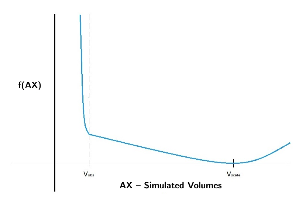
Figure 17: Partial Trip Cost Function Graph
When using partial trip data in the dynamic estimation procedure, Analyst Drive appends an additional term to the cost function represented mathematically by the vector function
where Vobs is the observed partial trip count volume, Vscale is the observed partial trip count volume multiplied by the count scaling factor (this gives the estimate for the actual partial trip count), AX is the simulated volume for the partial trip and Vc is the scaling factor confidence value as described above. The high order exponential term in Equation 12 creates an asymptotic boundary near Vobs, the observed partial trip count value, attempting to force the estimation procedure to keep the simulated partial trip volume to at least this value. The minimum of the function occurs at Vscale which represents the estimate for the true total partial trip volume. Figure 17 provides a visual representation of this cost function. Of note is the asymptote that forms just before the value of Vobs which attempts to force the simulated partial trip volume to be at least the observed count value. The minimum of the function occurs when AX = Vscale.
From a theoretical standpoint, the cost function used here for including partial trip data in the dynamic estimation procedure is rather forgiving toward the aspect of predicting the scaling factor by creating a shallow well around the minimum point AX = Vscale, but at the same time enforces a minimum boundary for the more known quantity that is the actual detector count. This flexibility can be invaluable in the case that scaling factors lead to conflict with other more precise input data. Having covered the theoretical aspects we will now discuss using partial trip data in Analyst Drive.